DCGAN
TF-GAN on TPUs Tutorial
- Tutorial authors: joelshor@google.com, westbrook@google.com, tomfeelslucky@google.com
현재 TPU에서 GAN 모델을 processing하는데 최적화되지 않음.
https://cloud.google.com/tpu/docs/faq
Compute Engine에서 생성적 적대 신경망(GAN)을 학습시킬 수 있나요?
GAN을 학습시키려면 일반적으로 생성자 학습과 구분자 학습을 번갈아 반복해야 합니다. 현재 TPU 실행 엔진은 단일 실행 그래프만 지원합니다. 그래프를 번갈아 실행하려면 완전히 다시 컴파일해야 하며 여기에는 30초 이상의 시간이 걸릴 수 있습니다.
가능한 해결책 중 하나는 항상 생성자와 구분자 모두의 손실 합계를 계산하는 것입니다. 단, 이러한 손실을 입력 텐서 두 개(g_w 및 d_w)로 곱해야 합니다. 생성자를 학습시켜야 하는 배치에서는 g_w=1.0 및 d_w=0.0으로 전달할 수 있고, 구분자를 학습시켜야 하는 배치에서는 반대로 전달할 수 있습니다.

이탤릭 볼드 이탤릭볼드
Overview
- TPUs 는 머신러닝 훈련과 인터페이스에 최적화된 칩셋이다.
- GAN 훈련은 많은 계산이 필요하지만 TPU를 이용하면 효율적으로 할 수 있다.
- MNIST 데이터셋으로 하면 직관적으로 이해하기 어렵기 때문에 CIFAR10 데이터셋으로 훈련한다.
- 50000 스텝에 대한 트레이닝이 TPU를 사용하면 약 10분이면 가능하다.
- DCGAN Architecture는 Deep Convolutional Generative Adversarial Network (DCGAN) 이다. 용어에 관해 더 많은 정보를 원하면 https://developers.google.com/machine-learning/glossary/#convolutional_neural_network 에 들어가서 확인한다.
- Learning objectives
- DCGAN의 generator 와 discriminator 의 이해
- TPU를 사용해서 CIFAR10 Dataset 훈련
- 생성한 이미지 확인
기본적으로 설치되어 있어야하는 패키지는 아래 코드 를 사용한다.
# Check that imports for the rest of the file work.
import os
import tensorflow as tf
!pip install tensorflow-gan
import tensorflow_gan as tfgan
import tensorflow_datasets as tfds
import tensorflow_hub as hub
import numpy as np
import matplotlib.pyplot as plt
# Allow matplotlib images to render immediately.
%matplotlib inline
# Disable noisy outputs.
tf.logging.set_verbosity(tf.logging.ERROR)
tf.autograph.set_verbosity(0, False)
import warnings
warnings.filterwarnings("ignore")
TPU or GPU detection
# Detect hardware, return appropriate distribution strategy
try:
    tpu = tf.distribute.cluster_resolver.TPUClusterResolver()  # TPU detection. No parameters necessary if TPU_NAME environment variable is set. On Kaggle this is always the case.
    print('Running on TPU ', tpu.master())
except ValueError:
    tpu = None

if tpu:
    tf.config.experimental_connect_to_cluster(tpu)
    tf.tpu.experimental.initialize_tpu_system(tpu)
    strategy = tf.distribute.experimental.TPUStrategy(tpu)
else:
    strategy = tf.distribute.get_strategy() # default distribution strategy in Tensorflow. Works on CPU and single GPU.

print("REPLICAS: ", strategy.num_replicas_in_sync)
Competition data access
TPUs read data directly from Google Cloud Storage (GCS). This Kaggle utility will copy the dataset to a GCS bucket co-located with the TPU. If you have multiple datasets attached to the notebook, you can pass the name of a specific dataset to the get_gcs_path function. The name of the dataset is the name of the directory it is mounted in. Use !ls /kaggle/input/ to list attached datasets.
GCP 버킷 접근
!git clone https://github.com/GoogleCloudPlatform/gcsfuse.git

!echo "deb http://packages.cloud.google.com/apt gcsfuse-bionic main" > /etc/apt/sources.list.d/gcsfuse.list
!curl https://packages.cloud.google.com/apt/doc/apt-key.gpg | apt-key add -
!apt -qq update
!apt -qq install gcsfuse
GCP Bucket 연동
!gcloud projects list  # 프로젝트 확인
!gsutil ls -L -b gs://bskim_bucket//  # 버킷이 있는지 확인

## gcsfuse 설치
!echo "deb http://packages.cloud.google.com/apt gcsfuse-bionic main" > /etc/apt/sources.list.d/gcsfuse.list
!curl https://packages.cloud.google.com/apt/doc/apt-key.gpg | apt-key add -
!apt -qq update
!apt -qq install gcsfuse

# colab에 버킷을 마운트시킬 폴더 생성
!mkdir folderOnColab

# GCP Bucket에서 colab으로 마운트
!gcsfuse bskim_bucket folderOnColab


# 잘 마운트 되었나 확인
!ls folderOnColab/                 # 폴더 안에 파일리스트
!cat folderOnColab/to_upload.txt   # 개별 파일 열어보기
Configuration
# Data access
GCS_DS_PATH = KaggleDatasets().get_gcs_path()

# Configuration
IMAGE_SIZE = [512, 512]
EPOCHS = 20
BATCH_SIZE = 16 * strategy.num_replicas_in_sync
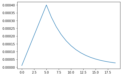
Custom LR schedule
LR_START = 0.00001
LR_MAX = 0.00005 * strategy.num_replicas_in_sync
LR_MIN = 0.00001
LR_RAMPUP_EPOCHS = 5
LR_SUSTAIN_EPOCHS = 0
LR_EXP_DECAY = .8

def lrfn(epoch):
    if epoch < LR_RAMPUP_EPOCHS:
        lr = (LR_MAX - LR_START) / LR_RAMPUP_EPOCHS * epoch + LR_START
    elif epoch < LR_RAMPUP_EPOCHS + LR_SUSTAIN_EPOCHS:
        lr = LR_MAX
    else:
        lr = (LR_MAX - LR_MIN) * LR_EXP_DECAY**(epoch - LR_RAMPUP_EPOCHS - LR_SUSTAIN_EPOCHS) + LR_MIN
    return lr

lr_callback = tf.keras.callbacks.LearningRateScheduler(lrfn, verbose=True)

rng = [i for i in range(EPOCHS)]
y = [lrfn(x) for x in rng]
plt.plot(rng, y)
print("Learning rate schedule: {:.3g} to {:.3g} to {:.3g}".format(y[0], max(y), y[-1]))
load dataset
train = pd.read_csv("/kaggle/input/digit-recognizer/train.csv")

Y_train = train['label'].values.astype('float32')
Y_train = tf.keras.utils.to_categorical(Y_train, 10)

X_train = train.drop(labels=['label'], axis=1)

# Normalize data
X_train = X_train.astype('float32')
X_train = X_train / 255
# Reshape data
X_train = X_train.values.reshape(42000,28,28,1)
X_train = np.pad(X_train, ((0,0), (2,2), (2,2), (0,0)), mode='constant')

X_train = np.squeeze(X_train, axis=-1)
X_train = stacked_img = np.stack((X_train,)*3, axis=-1)
모델 구성
# Need this line so Google will recite some incantations
# for Turing to magically load the model onto the TPU
def create_model():
    enet = efn.EfficientNetB3(
    input_shape=(32, 32, 3),
    weights='imagenet',
    include_top=False,
    )

    model = tf.keras.Sequential([
        enet,
        tf.keras.layers.Flatten(),
        tf.keras.layers.Dense(1024, activation="relu"),
        tf.keras.layers.Dropout(0.5),
        tf.keras.layers.Dense(10, activation='softmax')
    ])

    return model

with strategy.scope():
  model = create_model()
모델 컴파일
모델을 훈련하기 전에 필요한 몇 가지 설정이 모델 컴파일 단계에서 추가됩니다:
- 손실 함수(Loss function)-훈련 하는 동안 모델의 오차를 측정합니다. 모델의 학습이 올바른 방향으로 향하도록 이 함수를 최소화해야 합니다.
- 옵티마이저(Optimizer)-데이터와 손실 함수를 바탕으로 모델의 업데이트 방법을 결정합니다.
- 지표(Metrics)-훈련 단계와 테스트 단계를 모니터링하기 위해 사용합니다. 다음 예에서는 올바르게 분류된 이미지의 비율인 정확도를 사용합니다. ~~~python
model.compile(optimizer=’adam’, loss=’categorical_crossentropy’, metrics=[‘accuracy’])
## EfficientNet

### 모델 훈련
신경망 모델을 훈련하는 단계는 다음과 같습니다:

- 훈련 데이터를 모델에 주입합니다
- 모델이 이미지와 레이블을 매핑하는 방법을 배웁니다.
- 테스트 세트에 대한 모델의 예측을 만듭니다-이 예에서는 test_images 배열입니다. 이 예측이 test_labels 배열의 레이블과 맞는지 확인합니다.
- 훈련을 시작하기 위해 model.fit 메서드를 호출하면 모델이 훈련 데이터를 학습
- TPU에 맞춰서 Batch단위로 수행
~~~python

%%time

history = model.fit(
    X_train, Y_train,
    epochs=10,
    batch_size = 210,
    shuffle=True,
    verbose = 1
)
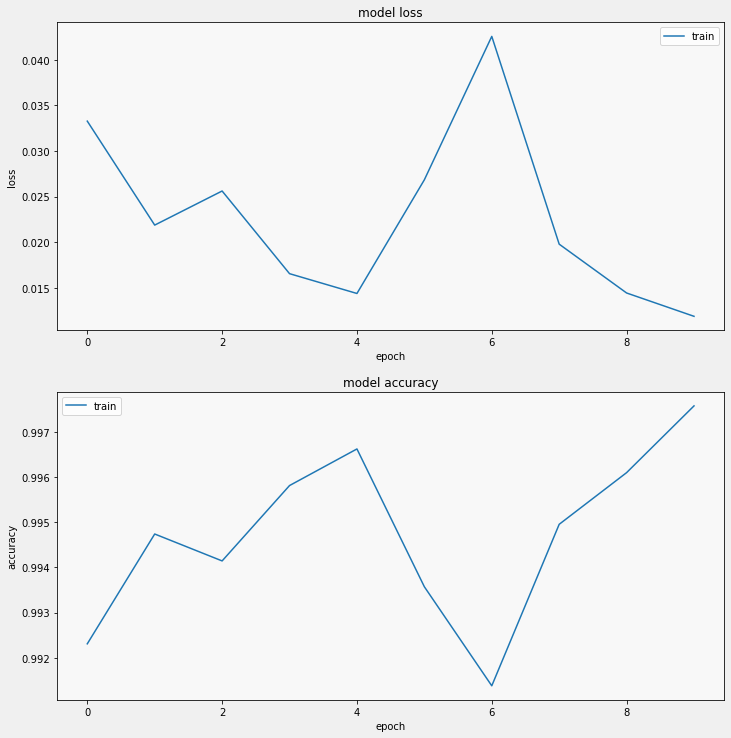
Loss, accuracy 확인
display_training_curves(history.history['loss'], 'loss', 211)
display_training_curves(history.history['accuracy'], 'accuracy', 212)