Home Prices Prediction Tutorial

https://www.kaggle.com/pmarcelino/comprehensive-data-exploration-with-python

이탤릭 볼드 이탤릭볼드

Workflow stages

Question or problem definition.
Acquire training and testing data.
Wrangle, prepare, cleanse the data.
Analyze, identify patterns, and explore the data.
Model, predict and solve the problem.
Visualize, report, and present the problem solving steps and final solution.
Supply or submit the results.

기본적으로 설치되어 있어야하는 패키지는 아래 코드 를 사용한다.

import pandas as pd
import numpy as np
from time import sleep

# visualization
import seaborn as sns
import matplotlib.pyplot as plt
%matplotlib inline

# machine learning
from sklearn.linear_model import LogisticRegression
from sklearn.svm import SVC, LinearSVC
from sklearn.ensemble import RandomForestClassifier
from sklearn.neighbors import KNeighborsClassifier
from sklearn.naive_bayes import GaussianNB
from sklearn.linear_model import Perceptron
from sklearn.linear_model import SGDClassifier
from sklearn.tree import DecisionTreeClassifier

data 가져오기

Train_Dir = 'training.csv'
Test_Dir = 'test.csv'
lookid_dir = 'IdLookupTable.csv'
train_data = pd.read_csv(Train_Dir)
test_data = pd.read_csv(Test_Dir)
lookid_data = pd.read_csv(lookid_dir)

data를 찍어보면 다음과 같이 나온다

print(train_data.head().T)

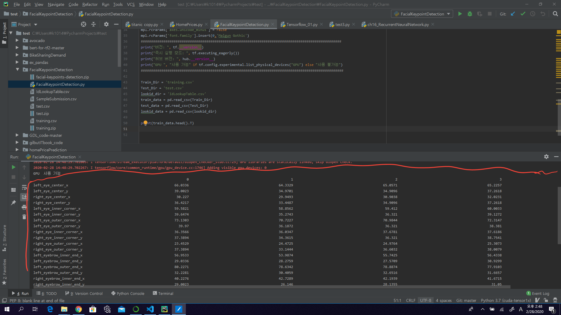
위와같은 카테고리로 되어있으며 data를 몇개 찍어보면 다음과 같다.

누락데이터 확인

print(train_data.isnull().any().value_counts())

True 28

False 3

dtype: int64

누락된 값 대체

train_data.fillna(method = 'ffill',inplace = True)
#train_data.reset_index(drop = True,inplace = True)

fillna 에 method를 ffill을 사용하여 이전 index의 값으로 누락값을 대체해준다. 다음 인덱스값으로 대체하려면 bfill을 사용하여 대체한다. False 31

dtype: int64

이미지 값 처리

현재 이미지 값이 238 236 237 238 240 240 239 241 241 243 240 23… 같은 형태로 되어있는데 이를 ‘ ‘(공백)을 기준으로 읽을 수 있도록 재 처리해준다.

imag = []
for i in range(0,7049):
    img = train_data['Image'][i].split(' ')
    img = ['0' if x == '' else x for x in img]
    imag.append(img)

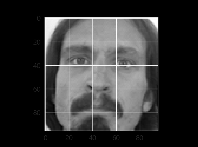
다음 처리된 이미지를 numpy를 이용하여 reshape를 해준다.

image_list = np.array(imag,dtype = 'float')
X_train = image_list.reshape(-1,96,96,1)

plt.imshow(X_train[0].reshape(96,96),cmap='gray')
plt.show()

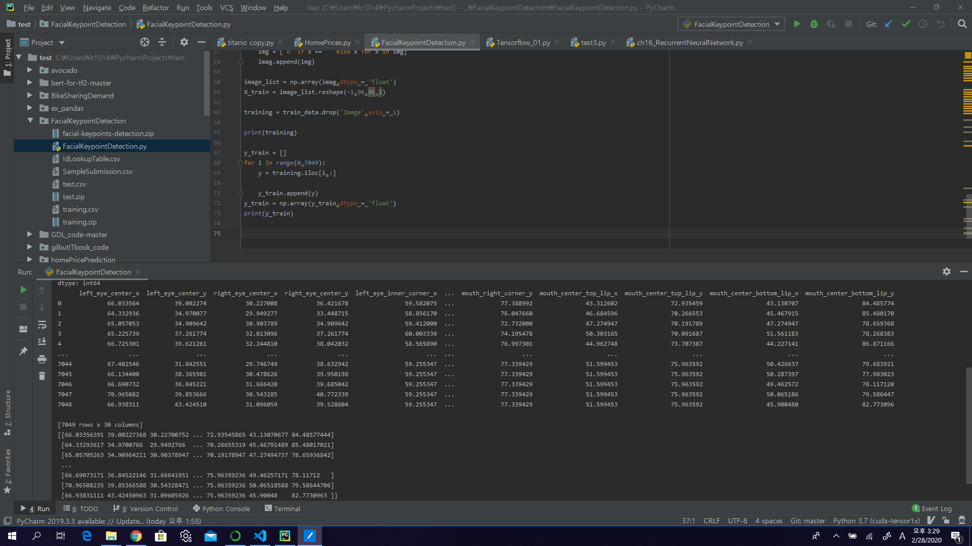
라벨 분리

y_train에 원 데이터에서 이미지를 제거하고 라벨만을 분리해서 넣어준다.

training = train_data.drop('Image',axis = 1)

y_train = []
for i in range(0,7049):
    y = training.iloc[i,:]

    y_train.append(y)
y_train = np.array(y_train,dtype = 'float')

모델 구성

신경망의 기본 구성 요소는 층(layer)입니다. 층은 주입된 데이터에서 표현을 추출합니다. 아마도 문제를 해결하는데 더 의미있는 표현이 추출될 것입니다.

대부분 딥러닝은 간단한 층을 연결하여 구성됩니다. tf.keras.layers.Dense와 같은 층들의 가중치(parameter)는 훈련하는 동안 학습됩니다.

model = tf.keras.Sequential([tf.keras.layers.Flatten(input_shape=(96,96)),
                         tf.keras.layers.Dense(128, activation="relu"),
                         tf.keras.layers.Dropout(0.1),
                         tf.keras.layers.Dense(64, activation="relu"),
                         tf.keras.layers.Dense(30)
                         ])

이 네트워크의 첫 번째 층인 tf.keras.layers.Flatten은 2차원 배열(96 x 96 픽셀)의 이미지 포맷을 96 * 96 = 9216 픽셀의 1차원 배열로 변환합니다. 이 층은 이미지에 있는 픽셀의 행을 펼쳐서 일렬로 늘립니다. 이 층에는 학습되는 가중치가 없고 데이터를 변환하기만 합니다.

픽셀을 펼친 후에는 두 개의 tf.keras.layers.Dense 층이 연속되어 연결됩니다. 이 층을 밀집 연결(densely-connected) 또는 완전 연결(fully-connected) 층이라고 부릅니다. 첫 번째 Dense 층은 128개의 노드(또는 뉴런)를 가집니다. 두 번째 (마지막) 층은 30개의 노드의 relu(relu) 층입니다. 이 층은 30개의 확률을 반환하고 반환된 값의 전체 합은 1입니다. 각 노드는 현재 이미지가 30개 클래스 중 하나에 속할 확률을 출력합니다.

모델 컴파일

모델을 훈련하기 전에 필요한 몇 가지 설정이 모델 컴파일 단계에서 추가됩니다:

손실 함수(Loss function)-훈련 하는 동안 모델의 오차를 측정합니다. 모델의 학습이 올바른 방향으로 향하도록 이 함수를 최소화해야 합니다.
옵티마이저(Optimizer)-데이터와 손실 함수를 바탕으로 모델의 업데이트 방법을 결정합니다.
지표(Metrics)-훈련 단계와 테스트 단계를 모니터링하기 위해 사용합니다. 다음 예에서는 올바르게 분류된 이미지의 비율인 정확도를 사용합니다.
```
model.compile(optimizer='adam', 
            loss='mean_squared_error',
            metrics=['mae'])
```

모델 훈련

신경망 모델을 훈련하는 단계는 다음과 같습니다:

훈련 데이터를 모델에 주입합니다
모델이 이미지와 레이블을 매핑하는 방법을 배웁니다.
테스트 세트에 대한 모델의 예측을 만듭니다-이 예에서는 test_images 배열입니다. 이 예측이 test_labels 배열의 레이블과 맞는지 확인합니다.
훈련을 시작하기 위해 model.fit 메서드를 호출하면 모델이 훈련 데이터를 학습합니다:
```
model.fit(X_train,y_train,epochs = 50,batch_size = 256,validation_split = 0.2)
```
256 batch size로 50 에폭만큼 train을 수행

모델 테스트

#preparing test data
timag = []
for i in range(0,1783):
    timg = test_data['Image'][i].split(' ')
    timg = ['0' if x == '' else x for x in timg]
    
    timag.append(timg)

테스트 이미지를 모델에 테스트 할 수 있도록 변환

timage_list = np.array(timag,dtype = 'float')
X_test = timage_list.reshape(-1,96,96,1) 

이미지 확인

plt.imshow(X_test[0].reshape(96,96),cmap = 'gray')
plt.show()

결과 확인

pred = model.predict(X_test)

제출 format으로 csv파일 내보내기

lookid_list = list(lookid_data['FeatureName'])
imageID = list(lookid_data['ImageId']-1)
pre_list = list(pred)
rowid = lookid_data['RowId']
rowid=list(rowid)
feature = []
for f in list(lookid_data['FeatureName']):
    feature.append(lookid_list.index(f))
preded = []
for x,y in zip(imageID,feature):
    preded.append(pre_list[x][y])
rowid = pd.Series(rowid,name = 'RowId')
loc = pd.Series(preded,name = 'Location')
submission = pd.concat([rowid,loc],axis = 1)
submission.to_csv('face_key_detection_submission.csv',index = False)

Facial Keypoint Detection