EfficientNet

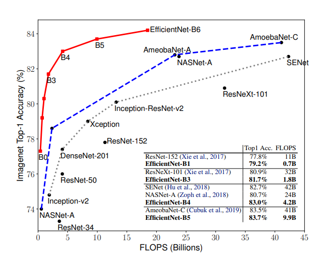
이 논문에서는 모델(F)를 고정하고 depth(d), width(w), resolution(r) 3가지를 조절하는 방법을 제안하고 있는데, 이때 고정하는 모델(F)를 좋은 모델로 선정하는 것이 굉장히 중요합니다. 아무리 scaling factor를 조절해도, 초기 모델 자체의 성능이 낮다면 임계 성능도 낮기 때문입니다. 이 논문에서는 MnasNet과 거의 동일한 search space 하에서 AutoML을 통해 모델을 탐색하였고, 이 과정을 통해 찾은 작은 모델을 EfficientNet-B0 이라 부르고 있습니다.

. EfficientNet Architecture

we develop our baseline network by leveraging a multi-objective neural architecture search that optimizes both accuracy and FLOP. which we name EfficientNet-B0
Starting from the baseline EfficientNet-B0, we apply our compound scaling method to scale it up with two steps
- STEP 1: we first fix φ = 1, assuming twice more resources available, and do a small grid search of α, β, γ based on Equation 2 and 3. In particular, we find the best values for EfficientNet-B0 are α = 1.2, β = 1.1, γ = 1.15, under constraint of α · β 2 · γ 2 ≈ 2
- STEP 2: we then fix α, β, γ as constants and scale up baseline network with different φ using Equation 3, to obtain EfficientNet-B1 to B7.

이탤릭 볼드 이탤릭볼드

Workflow stages

Question or problem definition.
Acquire training and testing data.
Wrangle, prepare, cleanse the data.
Analyze, identify patterns, and explore the data.
Model, predict and solve the problem.
Visualize, report, and present the problem solving steps and final solution.
Supply or submit the results.

기본적으로 설치되어 있어야하는 패키지는 아래 코드 를 사용한다.

import numpy as np
import pandas as pd
import matplotlib.pyplot as plt
import tensorflow as tf

print("Tensorflow version " + tf.__version__)

!pip install -q efficientnet

import efficientnet.tfkeras as efn

TPU or GPU detection

# Detect hardware, return appropriate distribution strategy
try:
    tpu = tf.distribute.cluster_resolver.TPUClusterResolver()  # TPU detection. No parameters necessary if TPU_NAME environment variable is set. On Kaggle this is always the case.
    print('Running on TPU ', tpu.master())
except ValueError:
    tpu = None

if tpu:
    tf.config.experimental_connect_to_cluster(tpu)
    tf.tpu.experimental.initialize_tpu_system(tpu)
    strategy = tf.distribute.experimental.TPUStrategy(tpu)
else:
    strategy = tf.distribute.get_strategy() # default distribution strategy in Tensorflow. Works on CPU and single GPU.

print("REPLICAS: ", strategy.num_replicas_in_sync)

Competition data access

TPUs read data directly from Google Cloud Storage (GCS). This Kaggle utility will copy the dataset to a GCS bucket co-located with the TPU. If you have multiple datasets attached to the notebook, you can pass the name of a specific dataset to the get_gcs_path function. The name of the dataset is the name of the directory it is mounted in. Use `!ls /kaggle/input/` to list attached datasets.

GCP 버킷 접근

!git clone https://github.com/GoogleCloudPlatform/gcsfuse.git

!echo "deb http://packages.cloud.google.com/apt gcsfuse-bionic main" > /etc/apt/sources.list.d/gcsfuse.list
!curl https://packages.cloud.google.com/apt/doc/apt-key.gpg | apt-key add -
!apt -qq update
!apt -qq install gcsfuse

GCP Bucket 연동

GCS_DS_PATH = KaggleDatasets().get_gcs_path() # you can list the bucket with "!gsutil ls $GCS_DS_PATH"

Configuration

# Data access
GCS_DS_PATH = KaggleDatasets().get_gcs_path()

# Configuration
IMAGE_SIZE = [512, 512]
EPOCHS = 20
BATCH_SIZE = 16 * strategy.num_replicas_in_sync

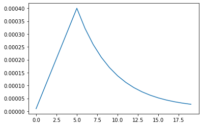
Custom LR schedule

LR_START = 0.00001
LR_MAX = 0.00005 * strategy.num_replicas_in_sync
LR_MIN = 0.00001
LR_RAMPUP_EPOCHS = 5
LR_SUSTAIN_EPOCHS = 0
LR_EXP_DECAY = .8

def lrfn(epoch):
    if epoch < LR_RAMPUP_EPOCHS:
        lr = (LR_MAX - LR_START) / LR_RAMPUP_EPOCHS * epoch + LR_START
    elif epoch < LR_RAMPUP_EPOCHS + LR_SUSTAIN_EPOCHS:
        lr = LR_MAX
    else:
        lr = (LR_MAX - LR_MIN) * LR_EXP_DECAY**(epoch - LR_RAMPUP_EPOCHS - LR_SUSTAIN_EPOCHS) + LR_MIN
    return lr
    
lr_callback = tf.keras.callbacks.LearningRateScheduler(lrfn, verbose=True)

rng = [i for i in range(EPOCHS)]
y = [lrfn(x) for x in rng]
plt.plot(rng, y)
print("Learning rate schedule: {:.3g} to {:.3g} to {:.3g}".format(y[0], max(y), y[-1]))

load dataset

train = pd.read_csv("/kaggle/input/digit-recognizer/train.csv")

Y_train = train['label'].values.astype('float32')
Y_train = tf.keras.utils.to_categorical(Y_train, 10)

X_train = train.drop(labels=['label'], axis=1)

# Normalize data
X_train = X_train.astype('float32')
X_train = X_train / 255
# Reshape data
X_train = X_train.values.reshape(42000,28,28,1)
X_train = np.pad(X_train, ((0,0), (2,2), (2,2), (0,0)), mode='constant')

X_train = np.squeeze(X_train, axis=-1)
X_train = stacked_img = np.stack((X_train,)*3, axis=-1)

모델 구성

# Need this line so Google will recite some incantations
# for Turing to magically load the model onto the TPU
def create_model():
    enet = efn.EfficientNetB3(
    input_shape=(32, 32, 3),
    weights='imagenet',
    include_top=False,
    )        
    
    model = tf.keras.Sequential([
        enet,
        tf.keras.layers.Flatten(),
        tf.keras.layers.Dense(1024, activation="relu"),
        tf.keras.layers.Dropout(0.5),
        tf.keras.layers.Dense(10, activation='softmax')
    ])
    
    return model

with strategy.scope():
  model = create_model()

모델 컴파일

모델을 훈련하기 전에 필요한 몇 가지 설정이 모델 컴파일 단계에서 추가됩니다:

손실 함수(Loss function)-훈련 하는 동안 모델의 오차를 측정합니다. 모델의 학습이 올바른 방향으로 향하도록 이 함수를 최소화해야 합니다.
옵티마이저(Optimizer)-데이터와 손실 함수를 바탕으로 모델의 업데이트 방법을 결정합니다.
지표(Metrics)-훈련 단계와 테스트 단계를 모니터링하기 위해 사용합니다. 다음 예에서는 올바르게 분류된 이미지의 비율인 정확도를 사용합니다. ~~~python

model.compile(optimizer=’adam’, loss=’categorical_crossentropy’, metrics=[‘accuracy’])

## EfficientNet

### 모델 훈련
신경망 모델을 훈련하는 단계는 다음과 같습니다:

- 훈련 데이터를 모델에 주입합니다
- 모델이 이미지와 레이블을 매핑하는 방법을 배웁니다.
- 테스트 세트에 대한 모델의 예측을 만듭니다-이 예에서는 test_images 배열입니다. 이 예측이 test_labels 배열의 레이블과 맞는지 확인합니다.
- 훈련을 시작하기 위해 model.fit 메서드를 호출하면 모델이 훈련 데이터를 학습
- TPU에 맞춰서 Batch단위로 수행
~~~python

%%time

history = model.fit(
    X_train, Y_train,
    epochs=10,
    batch_size = 210,
    shuffle=True,
    verbose = 1
)

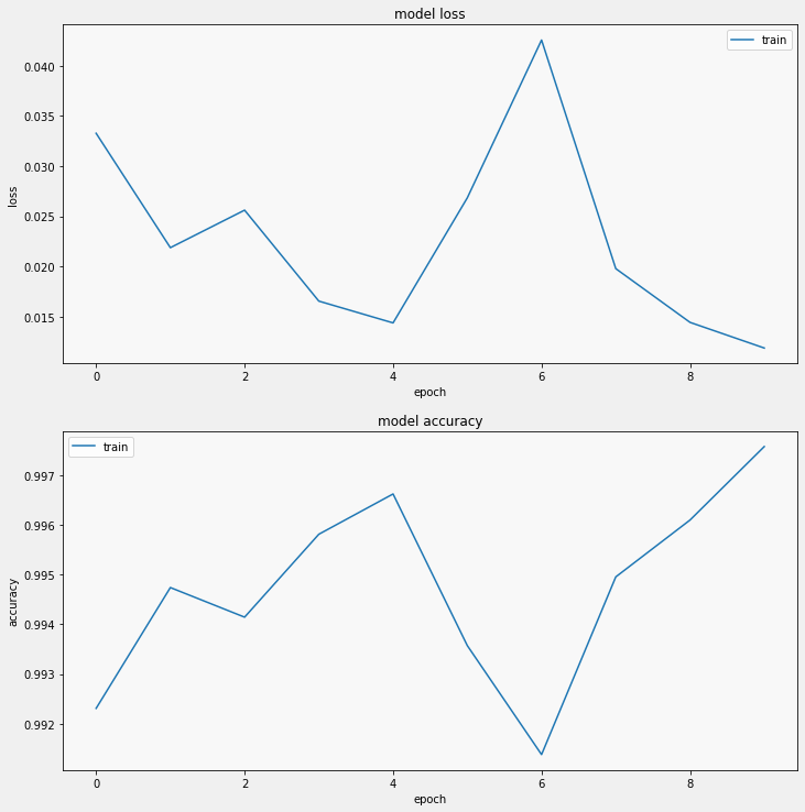
Loss, accuracy 확인

display_training_curves(history.history['loss'], 'loss', 211)
display_training_curves(history.history['accuracy'], 'accuracy', 212)

Kaggle TPU EfficientNet